Probability and Random Processes
Descriptive Statistics
Statistics
Statistics are the summarization of a set of data that has been collected, which demonstrates random variation. Extracting meaning from data.
Inferential Statistics
Inferential Statistics make inferences about a situation based on data, such as forecasting. Descriptive statistics can be the basis for inferences.
Representative Values
- Mean - The sum of all numbers in a list divided by the number of items in the list
- Median - The middle value in a list ordered from smallest to largest
- Mode - The most frequently occuring value in a list
- Range - [Min, Max]
- Variance - Average of deviation from the mean squared
- Standard Deviation - Measure of average absolute deviation
- Skewness - Measure of the shape of the distribution function
- Quantiles - Generalization of the median to percentiles
Observational vs. Experimental Data
Experimental Data involves manipulating objects to determine cause and effect in data. Observational Data refers to data extrapolated from naturally occurring events.
Basic Probability
Probability Calculus
Probability events have a total probability between zero and one.
An event that is sure to happen
The definition of probability for how often an event is observed can be related to the number of repetions of the experiment.
Counting the probability of heads in a set of coin tosses
The larger the number of repetiions, the higher accuracy with which we can predict the likelihood of an event happening.
Probability Model
Events
Events are elements in the set of possible outcomes in an experiment.
Sample Space
The set of all possible outcomes for an experiment.
The sample space for a dice roll
Subsets containing events in the sample space
The complement of a subset
Event Algebra
Or
The combination of two or more sets.
For
And
The set of events which occur in two or more sets.
For
- Mutual exclusion:
- Inclusion:
- Double complement:
- Commutation:
- Associativity:
- Distributivity:
- DeMorgan’s Law:
Probability of Events
- For any event
: - For the full set,
- If
and are Mutually Exclusive then - Axiom 3 can be extended:
Mutual Exclusivity refers to the fact that
Non-Mutually Exclusive
In cases where
This is due to the fact that in overlapping events, the same area of probability will be counted twice, though it has no statistical importance.
Non mutually exclusive OR
Complement of an Event
From expanding on these axioms, it can be seen that the complement of an event has a probability related to subtraction of itself from the sample space probability. If the chance of the event happening is known, the chance of an event not happening is found by subtracting this from absolute certainty.
The complement of a set versus the whole
Statistical Independence
Two events
Statistical independence
This refers to the fact that statistical data will happen independent of the preceding events. If you flip a coin, the probability of the next coin will be the same. If you take items from a bin, the probability of the next item being picked will go up, and is therefore dependent.
Repeated Independant Trials
From the rule of statistical independence, we can process repeated trials.
Coin Flips
Knowing that the probability of either event is 0.5, we can take the list of possible outcomes and calculate the probability.
Sampling with Replacement
In this case, we consider an event where an event occurring does not subtract from a finite amount of events, ie a coin flip. In the case of heads or tails, there aren't one less heads or tails. So it is as if we replace the event in our sample space.
Sampling without Replacement
Finite amounts of events that can be subtracted from the whole. If this event happens, it won't happen again, as if we have taken our card from a deck of cards and not placed it back in the deck.
Order of Outcomes When Sampling Without Replacement
Cases when its important what order events occur in. Did we draw the Ace of Spades within the first 3 draws? The number of each event is not important.
K-Tuples
When a trial is repeated
The Rule of Product
How many possibilities are there for the formation of
The Rule of Product
By this rule, the number of possibilities when rolling a dice, then flipping a coin, will be
Permutations of Unordered Outcomes
We no longer care in what order outcomes occur, we are only concerned with the number of outcomes of a certain sort across all trials.
This involves the number of ways we can choose
Permutations Without Replacement
- Experiments with two or more possible outcomes
- These trials can be repeated independently for
times - For each
th trial the outcome from the previous is removed - Probabilities change for each consecutive trial
The resulting set is ordered, but as mentioned before, we only care about the number of possible permutations from these elements.
The number of possible sets is
Example - The 13 cards of a suit in a deck of cards can be laid out in
If you want just
Consider this problem - Lisa has 13 different ornaments and wants to put 4 ornaments on her mantle. In how many ways is this possible?
Using the product rule, Lisa has 13 choices for which ornament to put in the first position, 12 for the second position, 11 for the third position, and 10 for the fourth position. So the total number of choices she has is
From this example, we can see that if we have
The notation for permutations is
Combinations of Non-Unique Outcomes
A combination is a way of choosing elements from a set in which order does not matter.
Consider the following example: Lisa has 13 different ornaments and she wants to give 3 ornaments to her mom as a birthday gift (the order of the gifts does not matter). How many ways can she do this?
We can think of Lisa giving her mom a first ornament, a second ornament, a third ornament, etc. This can be done in
There are
Rule of Combinations or Unordered Permutations
The notation for combinations is
Conditional Probability
A conditional probability is a probability that a certain event will occur given some knowledge about the outcome or some other event.
Rule of Conditional Probability
A simple example - A fair 12-sided die is rolled. What is the probability that the roll is a 3 given that the roll is odd?
This is
Because
Conditional Probability if statiscally independent
Bayes Theorem
When attempting to compute the conditional probability of two events, when only one event is known, the Bayes Theorem allows for a workaround.
Consider
Bayes Theorem
We can expand the equation in the numerator to demonstrate fully:
Therefore,
Total Probability
If
Total Probability
Knowing this,
Bayes General Rule
Total Probability, when $A_1$, $A_2$, $A_3$ form a partition
Random Variables
Random variables deal with a function
Discrete Probabilty Distributions
Discrete random variables involve events with a discrete set of values.
Probability Mass Function
The Probability Mass Function, or PMF
For a given value
Consider
Bernouli Random Variable
A Bernoulli RV is a discrete variable which will only produce values of
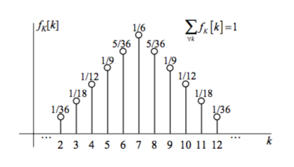
Binomial Random Variable
The Bernoulli concept can be extended with combinatorics, for example in the base of binary transmission error. When detecting the error in the first
As shown in earlier sections, there are
Geometric Random Variable
Geometric RVs concern a wait for an event to happen. Should the expected event be given
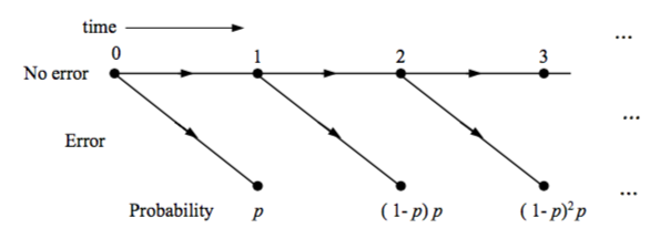
Geometric Random Variable PMF (0 $\leq$ k $<$ $\infty$)
Poisson Random Variable
For a situtation where revents occur randomly at a given rate
Poisson Random Variable PMF
Note that for finding the probability of an event occurring after time
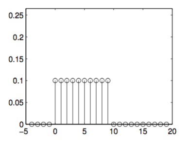
Uniform Random Variable
When all events are equally likely, the probability of each can be found easily from the uniform random variable PMF.
Uniform Distribution
Continous RVs and Their Distributions
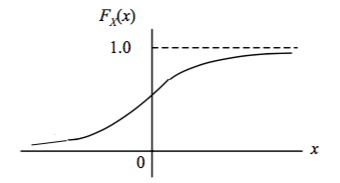
For values which can take on a continuum of values, such as voltage, velocity, and mass, new tools are used to analyze their probability. The probability of these events is determined using the Cumulative Distribution Function or CDF, which is written as
By this notation we can see that by following the graph from left to right, the probability of the event occuring to the left of value
When finding the probability of a value occurring between points
CDF Probability Within a Range (b $>$ a)
The Probability Density Function or PDF is a derivative of the CDF that can also be used to find this probability:
CDF Probability Within a Range (b $>$ a) From Integration
This can be seen to be similar to the Probability Mass Function, as it will integrate over its full range to
To use the PDF to find the probability of a number
PDF Probability Within a Range ($a < a + \Delta x$)
Integrating over a range (
Common Continuous RVs
Exponential Random Value
An extension of the Geometric Random Variable to the continuous realm, this represents a continuous graph of wait times where again
Its PDF follows
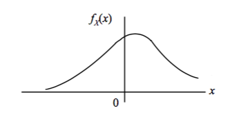
Gaussian RV
The Gaussian or "normal" random variable arises naturally in numerous cases. It can be defined by its mean,
The Gaussian PDF
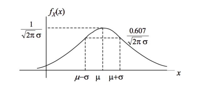
The square of the standard deviation,
The standard form of the PDF, centered at
The Standard Gaussian Function
And as with any other CDF,
These
Gaussian Q Values
In cases where the probablity of values at either tail of a Gaussian is required, such as
The Gaussian Q Function
When a value
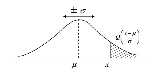
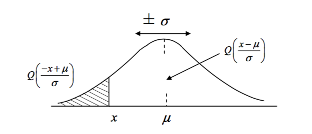
The Gaussian Q Function
The Gaussian Q Function with Negative Argument
Expectation
Expecation can be considered the average of the expected values in a sample space, where the values are weighted by their probability and summed.
Expectation of a Discrete RV
For continuous random variables, when the PDF exists, the expectation can be calculated whenever the variable converges absolutely:
Expectation of a Continuous RV
An important feature of the expectation is its invariance.
Moments
The moment is the produced when the
Continous Moment
Discrete Moment
The first moment is the mean, and each further
Central Moments
The Central Moment is a mean of a random variable not centered at 0. Of particular importance is the variance, the square root of which will grant the width of the distribution.
The 2nd Central Moment
The mean of $X$
The Standard Deviation is represented as
Also note,
Entropy
From the topic of information encoding, it was found that the definition of information for an event
And the average of information for two exclusive events
The definition of average information is in fact an expectation for two events that form a partition of a sample space.
For a partition
or,
Multiple Random Variables
Discrete Random Variables
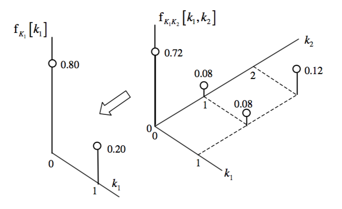
The Joint PMF
Joint probability distribution can be thought of as
Or as
A relationship can be deterministic, such as
Joint Probabilities refers to the probability of two variables taken together, such as
Recall from single random variable discussion, the PDF is the derivative of the CDF. Therefore, for cases where there are multiple variables:
For continuous distributions, the variables
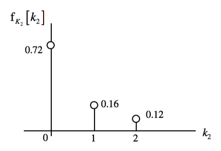
From each joint distribution, individual distributions for each variable, or \textbf{Marginal Distributions} can be found. These are simply the PDFs of the individual random variables found in earlier sections.
Independant Random Variables
From earlier in the course, events were defined as independent if
Notice that this is a special condition for random variables and does not apply in general! In particular, if two random variables are not independent, there is no way that the joint PMF can be inferred from the marginals. In that case the marginals are insufficient to describe any joint properties between
Continuous Random Variables
Joint Distributions
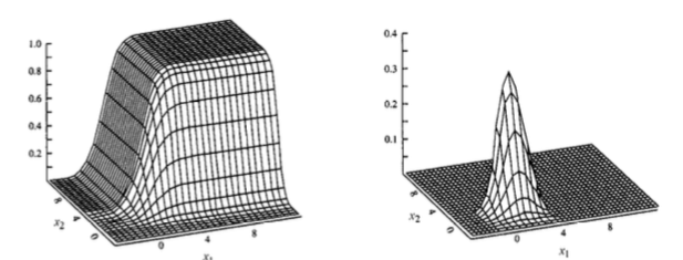
CDF:
PDF:
Joint continuity can be proven if the PDF evaluates to 1.
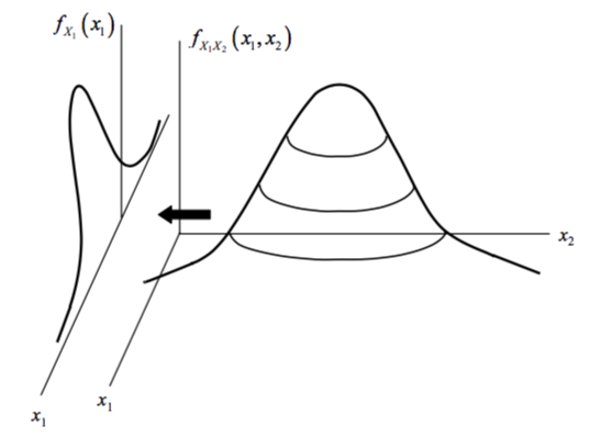
Marginal PDFs
Similar to the marginal PMF, each distribution
Correlation
Correlation is defined as the similarity between two random variables
The correlation is calculated using the expectation, worked out as the expectation for
The correlation can be misleading if both
Where
Note - Covariance is similar to variance, in that variance is a measure of how to the outcome of
Also similarly to variance:
Correlation Coefficient
If comparing the correlation of one of pair of random variables to the correlation of another pair of random variables, both can be normalized based on their standar deviations:
Where
Invariance of Expectation
If a random variable
Then moments for
Sum of Multiple RVs
Because the expectation
Therefore, because variance will distribute via multiplication:
PDF for
Begin by finding the CDF in a method similar to discrete RVs:
Note the limit of integration for the
The PDF can be obtained from this because
Because
If the two RVs are independent,
Notes on Sums of Independent RVs
- When
and are independent, = 0 and = + , while - If
and have the same distribution,
Sums of Dependent RVs
In the case of
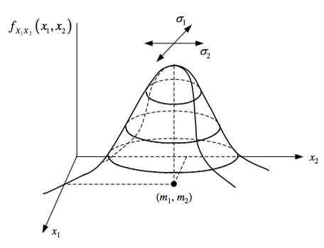
Bivariate Gaussian
Two joint RVs with Gaussian characteristics together will have a joint Gaussian characteristic, called bivariate or multi-variate for more than 2.
Limit Theorems
In other terms, when the number of trials approach large numbers, the mean of the trials will be